Visualizing logistic regression: from a line to a probability

Introduction

The perceptron asks a harsh question: which side of the line are you on? That is a useful question, but real decisions rarely come in pure yes-or-no form. A clinician does not want “sick” or “not sick” with no middle ground. A spam filter does not want to flip a coin on every borderline email. What we usually want is a probability: how confident should I be that this point belongs to class 1?

That is the job of logistic regression, one of the oldest and most important models in machine learning. It is a linear classifier at heart, just like a perceptron, but it wraps its linear score in a sigmoid so the output lives in $(0, 1)$ instead of jumping between $-1$ and $+1$. I think it is the perfect next step after staring at lines and gradients: same geometry, softer predictions, and a loss function that finally matches the thing we care about.

To understand logistic regression, I like to start the way I start most ML ideas: draw it. Once you can see the boundary, the sigmoid, and the update rule in the same picture, the whole model stops feeling like a formula sheet and starts feeling like a mechanism.

Logistic regression still splits the plane with a line, but it assigns graded probabilities on each side instead of a hard label.

Which side of the line?

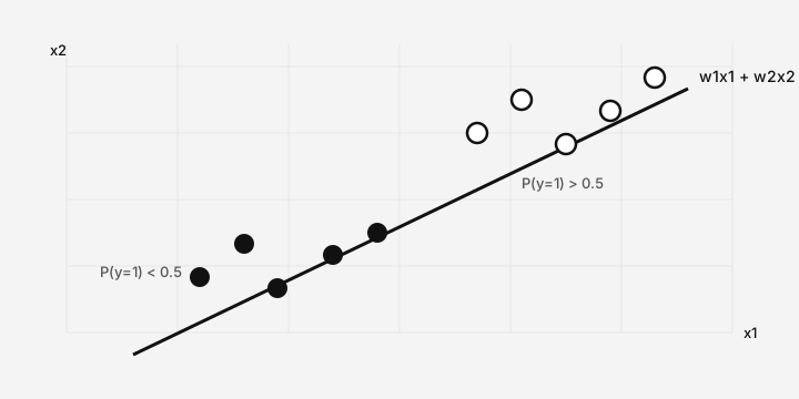
Suppose our data lives in 2D and we have a line

\[w_1 x_1 + w_2 x_2 + b = 0.\]

If you have seen the perceptron, this should feel familiar. The perceptron uses the sign of the score $z = w_1 x_1 + w_2 x_2 + b$ to emit $+1$ or $-1$. Logistic regression uses the same score, but passes it through a sigmoid:

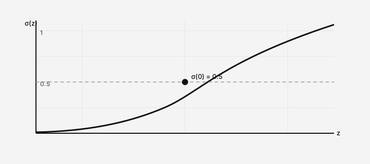
\[\sigma(z) = \frac{1}{1 + e^{-z}}.\]

The output is interpreted as $P(y=1 \mid x)$.

Note This is assuming the weights are oriented so that larger scores mean class 1. If you flip the signs of $w$ and $b$, the line stays the same but the class labels swap. You will see that happen if you train from a bad initialization in the playground below.

Intuitively, if a point sits far above the line in the positive-score region, then $z$ is large and $\sigma(z)$ is near 1. If it sits far below, $\sigma(z)$ is near 0. Points hugging the line get probabilities near 0.5, which is exactly the behavior we want when the world is ambiguous.

The sigmoid squashes any real score into the interval (0, 1).

Info Multiple proofs of the sigmoid’s shape and limits are collected in MIT’s Intro to ML classification notes (PDF). I kept returning to it while writing this post.

Drag the slider below and watch a raw score turn into a probability. This is the entire “activation” step of the model in one function.

Measuring wrongness with cross-entropy

If the model outputs a probability, we need a loss that punishes confident mistakes harshly. Mean squared error is a bad fit here: it plateaus in unhelpful ways and pushes probabilities in weird directions.

The standard choice is binary cross-entropy. For one example with true label $y \in {0,1}$ and prediction $\hat{y} = \sigma(z)$:

Key Point: $L(y, \hat{y}) = -\Big[y \log \hat{y} + (1-y)\log(1-\hat{y})\Big].$

Read that slowly. If $y=1$ and the model predicts 0.01, the first term blows up. If $y=0$ and the model predicts 0.99, the second term blows up. Correct confident predictions are cheap. Uncertainty is tolerated. Confident wrongness is expensive. That is the behavior you want from a classifier.

Here is the whole training loop in a few lines of Python, which is how I first made the idea click:

import numpy as np

def sigmoid(z):
    return 1 / (1 + np.exp(-z))

def train_step(X, y, w, b, lr=0.1):
    z = X @ w + b
    preds = sigmoid(z)
    error = preds - y
    grad_w = (X.T @ error) / len(y)
    grad_b = error.mean()
    w -= lr * grad_w
    b -= lr * grad_b
    loss = -np.mean(y * np.log(preds + 1e-8) + (1 - y) * np.log(1 - preds + 1e-8))
    return w, b, loss

Nothing exotic is happening. We compute predictions, measure how far they are from the labels, and nudge the weights downhill on the loss surface.

The update rule, stated like an algorithm

Geometrically, logistic regression is still about moving a line. Algebraically, each misclassified or under-confident point contributes a gradient that pushes the weights to increase $z$ for class-1 points and decrease it for class-0 points.

for each epoch:
    for each point (x, y):
        z  <- w · x + b
        p  <- sigmoid(z)
        error <- p - y
        w  <- w - lr * error * x
        b  <- b - lr * error

Compare that to the perceptron update: if a point is misclassified, nudge the weights by the input features. Logistic regression nudges on every point, but the nudge size depends on how wrong the probability was, not just whether the hard label was wrong. That small change is what makes the model smooth enough to optimize with calculus.

Tip If training looks stuck, check the learning rate first. Too small and the boundary crawls. Too large and the loss oscillates or diverges. The playground below is deliberately sensitive so you can feel that tradeoff.

Try it yourself

This widget is a tiny logistic regression trainer in 2D.

1. Choose hollow or filled dots.
2. Click the plot to place a few of each (hollow on one side, filled on the other).
3. Press Train. The gray background is predicted probability; the dashed line is the decision boundary.

Start with Reload demo if you want sample data already on the canvas.

One neuron, one idea

Once you write logistic regression as a weighted sum followed by a sigmoid, you have written down a single artificial neuron.

One neuron: weighted sum, sigmoid activation, probability out.

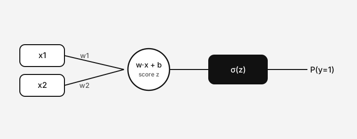
That is not just notation. A one-layer neural network for binary classification is logistic regression. Stack many of these neurons, add non-linearities between layers, and you are building the same object at larger scale. The sigmoid in this post is one activation function among many, but the pattern, linear score then non-linear squashing, is the repeating motif of modern deep learning.

Note Logistic regression still requires data that is roughly linearly separable if you want a clean decision boundary. For the classic XOR pattern, no single line works. That limitation is exactly why multi-layer networks exist.

What I like about this model

Logistic regression is old, which makes it easy to underestimate. But it is the cleanest place I know to connect four ideas that show up everywhere in ML: a boundary in feature space, outputs you can calibrate and threshold, gradient descent on a smooth loss, and one neuron as a building block.

If you are learning this for the first time, my advice is to play with the playground until the boundary motion feels predictable. Then re-read the update rule and notice how each term exists to fix a specific kind of mistake. That is the habit that turns formulas into intuition.

If you want to go deeper next, compare this post to a hard-margin classifier like the perceptron, or to the gradient-descent view of training in my earlier post on learning loops. The models change. The picture usually does not.

Sources

• MIT Intro to Machine Learning classification chapter (PDF)
• Andrew Ng, CS229 Lecture Notes: Classification and Logistic Regression
• Bishop, Pattern Recognition and Machine Learning, Section 4.3
• 3Blue1Brown, neural network series (excellent geometric intuition for activation functions)